• Complex Analysis: #4 Cauchy`s Theorem (simplest version)

Theorem 1
Let G ⊂ ℂ be a region, and assume that the function f : G → ℂ has an antiderivative (auf deutsch: Stammfunktion) F : G → ℂ with F' = f. Let γ be a closed path in G (that is, a continuous, closed, piecewise continuously differentiable path). (Closed means that γ(t₀) = γ(t₁).) Then ∫_γ f(z)dz = 0.

Proof

Since every polynomial has an antiderivative, it follows that the path integral around a closed path for any polynomial is zero.

Of course this is all a bit too trivial. So let’s call the following theorem the simplest version of Cauchy’s integral theorem.


Theorem 2
Let Q be a (solid) triangle in the complex plane. Assume that Q ⊂ G ⊂ ℂ, and take f : G → ℂ to be an analytic function. Let γ be the closed path traveling around the three sides of Q. Then ∫_γ f(z)dz = 0.

Proof
We may assume that γ begins and ends in a corner of Q — for example the “lowest” corner γ in the complex plane. If the lower side of Q is parallel to the real number axis, then take the right-hand corner on that side. Let us now divide the sides of Q in half, connecting the half-way points with straight line segments, thus creating four equal sub-triangles, Q₁, . . . , Q₄. Let γ_j be the path traveling around the boundary of Q_j, for j = 1, . . . , 4. Again we may assume that each γ_j begins and ends in the bottom right corner of it’s triangle. So we have

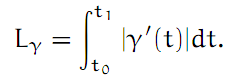
Assume further that each of these paths is parameterized in the simplest way possible, so that |γ'| = 1 and |γ_j'| = 1 for all the j. Therefore L_γ is the sum of the lengths of the three sides of the triangle Q, and L_γj = L_γ/2 for each of the j.

Let’s say that γ₁ is one of the numbers between one and four such that the value of

is the greatest. Then we certainly have

The next step is to concentrate on the triangle Q_j1. As with Q, we subdivide Q_j1 into four equal sub-triangles and we take paths around their boundaries. Choose Q_j2 to be one of these sub-triangles of Q_j1 which is such that the value of

is the greatest. Here γ_j2 is the path around the boundary of Q_j2. Now we have L_γj2= L_γ/4, and

This whole process is continued indefinitely, so that we obtain a sequence of triangles, becoming smaller and smaller, converging to a point, z₀ ∈ Q say,

Q ⊃ Q_j1⊃ Q_j2 ⊃ · · · → z₀ ∈ Q. 

For each n we have L_γjn= L_γ/2ⁿ and

But we have assumed that f is analytic, in particular it is differentiable at the point z₀. Thus we can write

f(z) = f(z₀) + f '(z₀)(z − z₀) + χ(z),

for points z in G, where χ : G → ℂ is a continuous function with

So let ∈ > 0 be arbitrarily given. Then there exists some δ > 0 such that |χ(z)| < |z − z₀| for all z with 0 < |z − z₀| < δ.

Now we need only choose n so large that |z − z₀| < δ for all z ∈ Q_jn. For such z we have

On the other hand, again since the length of L_γjnis L_γ/2ⁿ, we have

Bearing in mind Theorem 1 (and remembering that f '(z₀) is simply a constant complex number), we conclude that

Since ∈ was arbitrary and L_γ remains constant, we conclude that ∫_γ f(z)dz = 0.

But now Theorem 2 can be turned around, and we obtain (almost) the converse.


Theorem 3
Assume G ⊂ ℂ is a region and f : G → ℂ is a continuous function. Assume furthermore that for any solid triangle Q contained in G we have ∫_γ f(z)dz = 0, where γ is the path around the triangle. Then f has an antiderivative in every open disc contained in G. That is, let U = {z ∈ ℂ : |z − z_*| < r} be some such disc, where z_* is a complex number (the middle point of the disc) and r > 0 is the radius of the disc. Then there exists F : U → ℂ with F'(z) = f(z) for all z ∈ U.

Proof
By replacing f with the function f_*, where f_*(z) = f(z − z_*), we obtain the situation that z_* = 0. Clearly, if the theorem is true for f_*, then it is also true for f. Therefore, without loss of generality, we may simply assume that z_* = 0.

Within U the function F is defined to be

Here, α_z is the straight line from 0 to z, that is, α_z(t) = tz. To show that F really is an antiderivative to f in U, let z₀ be some arbitrary point of U and let z be some other point of U. Let β be the straight line connecting z₀ to z. That is, β(t) = (1 − t)z₀ + tz. Being a triangle, the integral of f around the path from 0 out to z, then from z to z₀ then from z₀ back to 0 must itself be zero. That is,

Looking at the definition of the path integral, we see that

Combining this theorem with Theorems 1 and 2, we see that if D ⊂ G is a closed disc, and γ is the circle of it’s boundary, then  ∫_γ f(z)dz = 0, for any analytic function defined in the region G. In fact, if γ is any (piecewise continuously differentiable and continuous) closed path contained within this disc-like G, then  ∫_γ f(z)dz = 0. For example we can look at a rectangle [a, b] × [c, d] contained within G. Since the rectangle can be taken to be a union of two triangles, attached along one side, we see that also the path integral around the rectangle must be zero.

More generally, the following theorem will prove to be useful.


Theorem 4
Let Q = {x + iy : 0 ≤ x, y ≤ 1} be the standard unit square in ℂ. Take ζ to be the standard closed path, traveling around the boundary of Q once in a counterclockwise direction, beginning and ending at 0. Assume that a continuously differentiable mapping ϕ : Q → ℂ is given, such that ϕ(Q) ⊂ G, a region where an analytic function f : G → ℂ is defined. Let γ = ϕ ◦ ζ be the image of ζ under ϕ. Then ∫_γ f(z)dz = 0.

Proof.
Since Q is compact, ϕ(Q) is also compact. Therefore it can be covered by a finite number of γ open discs in G. But Q can now be partitioned into a finite number of sub-squares Q₁, . . ., Q_n such that ϕ(Q_j) is in each case contained in a single one of these open discs. The theorem then follows by observing that the path integral around each of these sub-square images must be zero.

 Note:-
[The inverse images of the open discs in Q form a finite open covering V₁, . . ., V_m of Q. A sequence of partitions of Q can be obtained by cutting it along horizontal and vertical lines spaced 1/n apart, for each n ∈ ℕ. Can it be that for each of these partitions, there exists a sub-square which is not contained completely in one of the open sets V_k? But that would mean that there exists a limit point q ∈ Q such that for every ∈ > 0, there are infinitely many of these sub-squares contained within a distance of from q. However q ∈ V_k, for some k, and since V_k is open, there exists an ∈-neighborhood of q contained entirely within V_k, providing us with the necessary contradiction.]

A special case is the following.


Theorem 5
Let D₁ and D₂ be closed discs in ℂ such that D₂ is contained in the interior of D₁. Let γ_j be the closed path going once, counterclockwise, around the boundary of D_j, j = 1, 2. Let G ⊂ ℂ be a region containing D₁\D₂ and also containing the boundary of D₂. Assume that f : G → ℂ is analytic. Then ∫_γ1 f(z)dz = ∫_γ2 f(z)dz.

Proof
The annulus between D₂ and D₁ can be taken to be the image of the unit square under a continuously differentiable mapping.

A convenient notation for this situation is the following. Let γ : [0, 1] → ℂ be the path γ(t) = z₀ + re^2πit . Then we simply write

With this notation, we can say that if the analytic function f is defined in a region containing the annulus {z ∈ ℂ : r ≤ |z| ≤ R}, then we must have

• Complex Analysis: #3 Path Integrals

Let t₀ < t₁ be two real numbers. Then a continuous mapping γ : [t₀, t₁] → G ⊂ ℂ is a path in the region G of ℂ. In the analysis lecture we learned that γ is rectifiable if a number L exists such that for all ∈ > 0, a δ > 0 exists such that for every partition t₀ = a₀ < a₁ < · · · < a_n = t₁ which is such that a_j+1 − a_j < δ for all j, we have

Let γ(t) = γ_r(t) + iγ_i(t), where γ_r, γ_i: [t₀, t₁] → ℜ are real-valued functions. Then we say that the path is continuously differentiable if both the functions γ_r and γ_i are continuously differentiable. In this case, γ' = γ_r' + iγ_i' is also a path in ℂ. [Thinking in terms of 2-dimensional real geometry, we can say that γ'(t) is the "tangent vector" to γ(t).] We also learned that continuously differential paths are always rectifiable, and we have

All of this has already been dealt with in the analysis lecture. For us now, the interesting thing is to think about path integrals through a region where a complex-valued function is given.


Definition 3
Let G ⊂ ℂ be a region, and let f : G → ℂ be a function. Furthermore, let γ : [t₀, t₁] → G be a differentiable path. Then the path integral of f along γ is

assuming it exists.

The integral here is simply the sum of the integrals over the real and the imaginary parts. It is not necessary to assume that γ is continuously differentiable, but we will assume that it is piecewise continuously differentiable. That is, there is a partition of the interval [t₀, t₁] such that it is continuously differentiable along the pieces of the partition. So from now on, we will (almost) always assume that all paths considered are piecewise continuously differentiable.

As an exercise (using the substitution rule for integrals), one sees that the path integral does not depend on the way the path is parameterized. The simplest case is that, say γ(t) = t. Then (taking t from 0 to 1) we just have ∫_γ f(z)dz = ∫₀¹ f(t)dt. Almost equally simple is the case that γ(t) = it. Then we have ∫_γ f(z)dz = i∫₀¹ f(it)dt.

Increasing the complexity of our thoughts ever so slightly, we arrive at the first version of Cauchy’s integral theorem.

• Complex Analysis: #2 Analytic Functions

Definition 1
Any non-empty connected  open set G ⊂ ℂ will be called a region.

(Recall that in ℜ², every open connected subset is also path-connected.) So we will generally be interested in functions f : G → ℂ defined in regions.

Definition 2
Let f : G → ℂ be given, and let z₀ ∈ G. If

exists, then it is the derivative of f at z₀. The function f will be called analytic in G if it is defined, and has a continuous derivative everywhere in G. The word holomorphic is also used, and it is synonymous with the word analytic.

As in real analysis, we have the simple rules for combining the derivatives of two functions f and g:

Nevertheless, there is a very big difference between the idea of a derivative in complex analysis, and the familiar derivative in real analysis. The reason for this is that a common limit must exist, regardless of the direction with which we approach the point z₀ in the complex plane. This leads to the Cauchy-Riemann differential equations.

Looking at the definition of the complex derivative, one immediately sees that it is really a special version of the total derivative (as in analysis 2) in ℜ². Thus, for ξ ∈ ℂ sufficiently small (that is |ξ| small), we have

f(z₀ + ξ) = f(z₀) + Aξ + |ξ|ψ(ξ), 

where A is a 2 ×2 real matrix, and lim_ξ→0 ψ(ξ) = 0. But what is A? It represents multiplication with the complex number f '(z₀) = a + ib, say. That is,

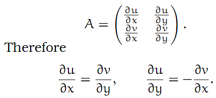
So what are these real numbers a and b? Let f(z) = u(z) + iv(z), where u, v : G → ℜ are real functions. Then writing z = x + iy, we have f(x + iy) = u(x + iy) + iv(x + iy). Identifying ℂ with ℜ², we can consider the partial derivatives of u and v. Since A is simply the Jacobi matrix of the mapping f at the point z₀, we must have

These are the Cauchy-Riemann equations. Another way to express this is to simply say that we must have

Thinking in geometrical terms, we see that if f is analytic, then it is a conformal mapping, at least at the points where f ' is not zero. That means that, locally, the mapping preserves angles. Looked at up close, the mapping is

Of course, as we have already seen, the rotation preserves orientation. Thus it is an element of the group SL₂ (R).

Another interesting detail is that the real and imaginary parts of an analytic function are themselves harmonic functions. Anticipating a later conclusion, let us assume that the parts of the analytic function f = u + iv are twice continuously differentiable. Since ∂u/∂x = ∂v/∂y and ∂u/∂y = −∂v/∂x, we have

Or, expressed in another standard form of notation,

u_xx + u_yy  = ∆u = 0. 

Here, ∆ is the Laplace operator. Similarly, we see that ∆v = 0.

All of this shows that we cannot simply choose any old smooth function f : G → ℂ and expect it to be analytic. On the contrary, there is a very great “rigidity”, which means that most smooth functions — even though they may be partially differentiable when considered as mappings of 2-dimensional Euclidean space — are not complex differentiable.


Examples

1. The first example is the nice and smooth function f(z) = f(x + iy) = x² + y². Here u_x = 2x and v_y = 0. But according to the Cauchy-Riemann equations, we must have u_x = v_y; that is, x = 0. This only holds along a single line in the complex plane ℂ. Therefore it certainly can’t hold in any region of ℂ (since regions are defined to be open), and thus f, despite all appearances of being a nice function, is definitely not analytic.



2. Having been cautioned by the previous example, let us try to construct an analytic function. For example, let us assume that u(x + iy) = x. What possibilities are there for v(x + iy)? Since u_x = 1 = v_y and v_y = 0 = v_x, it is clear that the only possibility is v(x + iy) = y + constant. So this is just the rather boring function f(z) = z + constant.



3. Thinking more positively, we have just seen that the simplest non-trivial polynomial, namely f(z) = z, is analytic throughout ℂ. Of course the simplest polynomial, f(z) = constant, is also analytic. But then, noting that we can use the sum and product rules for differentiation in complex analysis, we see that any arbitrary complex polynomial is analytic throughout ℂ. Indeed, z⁻ⁿ is also analytic (in ℂ \ {0}) for any n ∈ ℕ.

• Complex Analysis: #1 Complex Numbers

An “imaginary” number is introduced, called i (for imaginary)(sometimes j is also used in physics), which is declared to be a solution of the polynomial equation

x²+ 1 = 0.

The field of complex numbers is denoted by ℂ. We have

ℂ = {x + iy : x, y ∈ ℜ}. 

For z = x + iy, we also write Re(z) to denote the real part of z, namely the real number x. Also Im(z) = y is the imaginary part of z.

Let z₁ = x₁ + iy₁ and z₂ = x₂ + iy₂ be complex numbers. Then the addition and multiplication operations are given by

 z₁ + z₂ = (x₁ + x₂) + i(y₁ + y₂)

and

z₁ · z₂ = (x₁·x₂ − y₁·y₂) + i(x₁·y₂ − x₂·y₁).

The complex conjugate is z = x − iy (that is, z = x+i(−y)). Therefore the complex conjugate of z = z . We have |z|² = zz = x² + y². If z ≠ 0 (that is, either x ≠ 0, or y ≠ 0) then zz > 0, and we have

If z ≠ 0 then there are unique real numbers r > 0 and 0 ≤ θ < 2π such that x = r cos θ and y = r sin θ. So let u, v ∈ ℂ be non-zero numbers, and let

u = r(cos θ + i sin θ), 

v = s(cos ψ + i sin ψ). 

Then (remembering the rules for combining trigonometric functions), we see that

u · v = r · s(cos(θ + ψ) + i sin(θ + ψ)). 

If ℂ is identified with ℜ², the 2-dimensional real vector space, then we can identify any complex number z = x +iy. But for any two real numbers x and y, there exists a unique pair of numbers r ≥ 0, 0 ≤ θ < 2π, with x = r cos θ and y = r sin θ. (Obviously it is not quite unique for the number z = 0) So let u = s + it be some other complex number. Then

Thus we see that multiplication of complex numbers looks like an (orientation preserving) orthogonal mapping within ℜ² — combined with a scalar factor r.

More generally, let f : ℜ² → ℜ² be an arbitrary linear mapping, represented by the matrix

 How can this mapping be represented in terms of complex arithmetic? We have

Therefore, using the linearity of f, for z = x + iy we have

Therefore, if f(1) = −if(i), that is, if(1) = f(i), then the mapping is simply complex multiplication. On the other hand, if f(1) = if(i) then we have f(z) = w · z, where w = (f(1) + if(i))/2 ∈ ℂ is some complex number.

for a suitable choice of r and ψ. This is an orientation reversing rotation (again combined with a scalar factor r).

Now let u = a + ib and v = c + id. What is the scalar product <u, v>? It is

Therefore <z, z> = |z|², where |z| = √x² + y² is the absolute value of z = x + iy.

• Clausius Mossotti Equation | Static relative Permittivity | Polarization of Dielectric Materials

Total Polarization 
In the presence of electronic, ionic and dipolar polarization mechanisms, the average induced dipole moment per molecule p_av will be the sum of all the contributions in terms of the local field (effective field) acting on each individual molecule,

where α_e, α_i and α_d are the electronic, ionic and dipolar (orientational) polarizabilities. E_loc is the local field, the effective field, at the site of an individual molecule that causes the induced polarization. Each effect adds linearly to the net dipole moment per molecule which is a fact verified by experiments. Interfacial polarization cannot be simply added to the above as α_if E_loc because it occurs at interfaces and cannot be put into an average polarization per molecule in the bulk.

Further, the fields are not well defined at the interfaces. In the simplest case (valid for gases), we can take the local field to be the same field (average field in the sample). This means that E_loc = E and therefore polarization Since P = Np_av, where N is the number of atoms or molecules per unit volume,

where α is the polarizability of the molecule. In solids we have to consider the actual effective field acting on a molecule. In the case of electronic and ionic polarization, the local field for cubic crystals and isotropic materials (such as liquids) can be shown to be given by the Lorentz field

The dielectric constant ε_r under electronic and ionic polarizations is then given by the Clausius Mossotti equation,

where ε_r is the relative permittivity at low frequencies, α_e is the electronic polarization, N_i is the number of ions (or atoms) per unit volume exhibiting electronic polarization, α_i is the effective ionic polarizability per ion pair and N_i is the number of ion pairs per unit volume.

Above the frequencies for ionic polarization relaxation, only electronic polarization will contribute to the relative permittivity, which will be lowered to ε_rop (relative permittivity at optical frequencies) and given by

In the case of dipolar materials (orientational polarization), we cannot use the simple Lorentz local field approximation. That is, the Clausius-Mossotti equation does not work with dipolar dielectrics and the calculation of the local field is quite complicated.

Table 1 summarizes the various polarization mechanisms and the corresponding static (or very low frequency) dielectric constant, and gives typical examples where one mechanism dominates over others.

Table 1
Typical examples of polarization mechanisms.

1. Problem: Electronic polarizability of non-polar gases

 The electronic polarizability of the Ar atom is 1.7 × 10^-40 F m². What is the static dielectric constant of Ar gas at 1 atmosphere at room temperature (300 K)?  


Solution
To calculate ε_r we need the number of Ar atoms per unit volume, N. If P is the pressure, V is the volume and N′ is the total number of atoms, then the ideal gas law is

PV = (N′/N_A)RT 

where R is the gas constant and T is the absolute temperature and N′/N is the number of moles of gas. Then, P = NkT where N = N ′/V, is the number of atoms per unit volume and k = R / N_A, is the Boltzmann constant. Thus,

Using the Clausius-Mossotti equation, Equation (2), gives the same result because when Nα_e is small as in the case of gases, the Clausius-Mossotti equation simplifies to Equation (1). The reader can verify this by expanding Equation (2) in a series in terms of (Nα_e) and neglecting terms greater than the linear term. The dielectric constant of most gases is small for one major reason. The number of atoms or molecules per unit volume N is very small compared with the number of atoms or molecules in the liquid and solid states. Generally the dielectric constant of most nonpolar gases (including air) can be takes as 1, the same as vacuum except at very high pressures.




2. Problem: Electronic polarizability of a van der Waals solid

The electronic polarizability of the Ar atom is 1.7 × 10^-40 F m². What is the static dielectric constant of solid Ar (an FCC crystal below 84 K) if its density is 1.8 g cm^-3?


Solution
 To calculate ε_r we need the number of Ar atoms per unit volume N from the density d. If  M_at = 39.95 g mol^-1 is the relative atomic mass of Ar and N_A is Avogadro's number then we have,

The two values are different by about 17%. The simple relationship in Equation (1) underestimates the relative permittivity and would be appropriate for gaseous Ar.




3. Problem: Relative permittivity of ionic crystals

Consider a CsCl crystal which has the CsCl unit cell crystal structure (one Cs⁺–Cl^- pair per unit cell) with a lattice parameter (a) of 0.412 nm. The electronic polarizability of Cs⁺ and Cl^- ions are 3.35 × 10 ^-40 F m², and 3.40 × 10^-40 F m² respectively, and the mean ionic polarizability per ion pair is 6 × 10^-40 . What is the low frequency dielectric constant and that at optical frequencies?

Solution
The CsCl structure has one action (Cs⁺) and one anion (Cl^-) in the unit cell. Given the lattice parameter a = 0.412 × 10^-9m, number of ion pairs N_i per unit volume is

At high frequencies, that is near optical frequencies, the ionic polarization is too sluggish to allow ionic polarization to contribute to ε_r. Thus, ε_rop, relative permittivity at optical frequencies, is given by

Note that experimental values are ε_r = 7.20 at low frequencies and ε_rop = 2.62, very close to calculated values.




4. Problem: Dielectric constant of water (a dipolar liquid)

Given the static dielectric constant of water as 80, its density as 1 g cm^-3, calculate the permanent dipole moment p₀ per water molecule assuming that it is the orientational polarization of individual molecules that gives rise to the dielectric constant. Use both the simple relationship in Equation (1) and also the Clausius-Mossotti equation and compare your results with the permanent dipole moment of the water molecule which is 6.1 × 10^-30C m.  


Solution
We first need the number of H₂O molecules per unit volume. The molecular mass, M_mol is 18 × 10^-3 kg mol^-1, its density d is 10³kg m^-3. The number of H₂O molecules per unit volume N_d is

This is three times greater than the actual permanent dipole moment of H₂O (∼ 6 × 10^-30 C m). On the other hand, if we use the Clausius-Mossotti equation we find p₀ = 3.1 × 10^-30 C m, which is half the actual permanent dipole moment of H₂O. Both are unsatisfactory calculations. The reasons for the differences are two fold. First is that the individual H₂O molecules are not totally free to rotate. In the liquid, H₂O molecules cluster together through hydrogen bonding so that the rotation of individual molecules is then limited by this bonding. Secondly, the local field can neither be totally neglected nor taken as the Lorentz field. A better theory for dipolar liquids is based on the Onsager theory which is beyond the scope of this document. Interestingly, if we use the actual p₀ = 6.1 × 10^-30 C m in the Clausius-Mossotti equation, then ε_r turns out to be negative, which is nonsense.





USEFUL DEFINITIONS  

Avogadro's number (N_A) is the number of atoms in exactly 12 grams of Carbon-12. It is 6.022 × 10²³. Since atomic mass is defined as 1/12 of the mass of the carbon-12 atom, N_A number of atoms of any substance has a mass equal to the atomic mass, M_at, in grams.  

Boltzmann’s constant k is the gas constant per atom or per molecule, that is, the gas constant divided by Avogadro’s number (k = R/N_A); k = 1.38 × 10^-23 J K^-1. (3/2kT is the mean kinetic energy associated with the translational motions of gas molecules in a gas cylinder at temperature T).

Clausius-Mossotti equation relates the dielectric constant (ε_r), a macroscopic property, to the  polarizability (α), a microscopic property.  

Dielectric is a material in which energy can be stored by the polarization of the molecules. It is a material that increases the capacitance or charge storage ability of a capacitor. Ideally it is a non-conductor of electrical charge so that an applied field does not cause a flow of charge but instead a relative displacement of opposite bound charges and hence polarization of the medium.

Dipolar (orientational) polarization arises when randomly oriented polar molecules in a dielectric are rotated and aligned by the application of a field so as to give rise to a net average dipole moment per molecule. In the absence of the field the dipoles (polar molecules) are randomly oriented and there is no average dipole moment per molecule. In the presence of the field the dipoles are rotated, some partially and some fully, to align with the field and hence give rise to a net dipole moment per molecule.  

Electronic polarization is the displacement of the electron cloud of an atom with respect to the positive nucleus. Its contribution to the relative permittivity of a solid is usually small.  

Ionic polarization is the relative displacement of oppositely charged ions in an ionic crystal that results in the polarization of the whole material. Typically ionic polarization is important in ionic crystals below the infrared wavelengths.  

Polarization is the separation of positive and negative charges in a system so that there is a net electric dipole moment per unit volume.  

Relative permittivity (ε_r) or the dielectric constant of a dielectric is the fractional increase in the stored charge per unit voltage on the capacitor plates due to the presence of the dielectric between the plates (the whole space between the plates is assumed to be filled). Alternatively we can define it as the fractional increase in the capacitance of a capacitor when the insulation between the plates is changed from vacuum to a dielectric material keeping the geometry the same.  

Valence electrons are those electrons in the outer shell of an atom. As they are the farthest away from the nucleus, they are the first electrons involved in atom-to-atom interactions.





Important Note: This article was originally written by Safa Kasap. He reserves all rights. Use this article only for educational purpose. The document can be obtained at the author`s website.

• Expression for Conductivity of ionized gas (plasma) at low pressure

A plasma is an ionized gas. As a rule, plasmas contain free electrons and positive ions. Since the ions are more massive than the electrons, the current is carried almost exclusively by the electrons.

At low pressure, we can ignore the collisions between the electrons and the gas molecules, and hence energy losses.

Considering a plane electromagnetic wave (EM wave) propagating, the motion of the charge depends almost entirely on the electric field (E-field).

The conductivity of the gas is given by where Jt is the electron current density.

Actually, Jt is the sum if all ions in the gas.

where Ni is the number of electrons or ions per metre cube, Qi is the charge of electrons or ions and dxi/dt (= vi) is the speed of the electron or ion along the x-axis.

Now, we require the velocity v of a free electron or ion of mass m subjected to an alternating electric field.

Note that the time derivative of velocity v here can be written as dv/dt = jwv ; assuming for example that v = v0 exp(jwt) where j represents the imaginary component, w the frequency and t the time.

Taking the expressions for the force, we obtain

v leads the field by 90⁰

Then, replacing this expression of v in Jt , taking the pure imaginary part (the "-90⁰") and equating the 2 equations for Jt, we get

As the mass of the ions is much larger than that of the electrons while the charge is of the same order of magnitude as that of the electrons, the contribution of the ions can be neglected.

Thus, the conductivity can be written in terms of the charge and mass of electrons only.

So, this is the simple expression that can be used to calculate the conductivity of the plasma.