FOLLOW US ON TWITTER
SHARE THIS PAGE ON FACEBOOK, TWITTER, WHATSAPP ... USING THE BUTTONS ON THE LEFT


YOUR PARTICIPATION FOR THE GROWTH OF PHYSICS REFERENCE BLOG

Wednesday, December 26, 2012

Plane Harmonic Wave Equations in Harmonic Isotropic Linear Stationary (HILS) medium

  • Plane Harmonic Wave Equations in Harmonic Isotropic Linear Stationary (HILS) medium

We`ll now derive the Plane Harmonic Wave Equations in Harmonic Isotropic Linear Stationary (HILS) medium from the Maxwell`s equations.

The general Maxwell`s equations are

Plane Harmonic Wave Equations in Harmonic Isotropic Linear Stationary (HILS) medium maxwell equation \center \overrightarrow{\triangledown }\cdot \overrightarrow{E} = \frac{\rho_{free}}{\varepsilon_0} \; \; \; \; \;\;\;\; (1)\\ \\ \\ \\ \overrightarrow{\triangledown }\cdot \overrightarrow{B} = 0 \; \; \; \; \;\;\;\; (2)\\ \\ \\ \\ \overrightarrow{\triangledown } \times \overrightarrow{E} = -\frac{\partial \overrightarrow{B}}{\partial t} \; \; \; \; \;\;\;\; (3) \\ \\ \\ \\ \\ \overrightarrow{\triangledown } \times \overrightarrow{B} = \mu\overrightarrow{J_{free}} + \frac{1}{c^2} \frac{\partial \overrightarrow{E}}{\partial t} \; \; \; \; \;\;\;\; (4)


For linearity and isotropy, we have

 Plane Harmonic Wave Equations in Harmonic Isotropic Linear Stationary (HILS) medium equation 1 \overrightarrow{D} = \varepsilon \overrightarrow{E}\; , \; \overrightarrow{B} = \mu \overrightarrow{H}\; , \; \overrightarrow{J_{free}} = \sigma  \overrightarrow{E}

We will use the following identity to obtain the wave equations

Plane Harmonic Wave Equations in Harmonic Isotropic Linear Stationary (HILS) medium curl curl identity \overrightarrow{\triangledown} \times (\overrightarrow{\triangledown} \times \overrightarrow{X})= \overrightarrow{\triangledown} (\overrightarrow{\triangledown}\cdot \overrightarrow{X}) - \overrightarrow{\triangledown}^2 \overrightarrow{X}


To derive the wave equation for E

Plane Harmonic Wave Equations in Harmonic Isotropic Linear Stationary (HILS) medium equation 5 \center \overrightarrow{\triangledown} \times (\overrightarrow{\triangledown} \times \overrightarrow{E})= \overrightarrow{\triangledown}(\overrightarrow{\triangledown}\cdot \overrightarrow{E}) - \overrightarrow{\triangledown}^2 \overrightarrow{E} \; \; \; \; \; \; \; \; (5)

Plane Harmonic Wave Equations in Harmonic Isotropic Linear Stationary (HILS) medium equation 6 \overrightarrow{\triangledown}^2 \overrightarrow{E} - \overrightarrow{\triangledown}(\overrightarrow{\triangledown}\cdot \overrightarrow{E}) = \frac{\partial}{\partial t}(\overrightarrow{\triangledown} \times \overrightarrow{B}) \; \; \; \; \; \; \; \; (6)

Plane Harmonic Wave Equations in Harmonic Isotropic Linear Stationary (HILS) medium equation 7 \overrightarrow{\triangledown}^2 \overrightarrow{E} - \overrightarrow{\triangledown}(\overrightarrow{\triangledown}\cdot \overrightarrow{E}) = \frac{\partial}{\partial t}(\mu\overrightarrow{J_{free}} + \varepsilon\mu \frac{\partial \overrightarrow{E}}{\partial t} ) \; \; \; \; \; \; \; \; (7)

replacing Jfree in the equation (7)

So, we get the wave equation for E

Plane Harmonic Wave Equations in Harmonic Isotropic Linear Stationary (HILS) medium equation 9 \overrightarrow{\triangledown}^2 \overrightarrow{E} -  \sigma\mu \frac{\partial \overrightarrow{E}}{\partial t} - \frac{1}{c^2} \frac{\partial^2 \overrightarrow{E}}{\partial t^2} =  \overrightarrow{\triangledown}(\frac{\rho_{free}}{\varepsilon_0})\; \; \; \; \; \; \; \; (9)


To obtain the wave equation for B in Harmonic Isotropic Linear Stationary (HILS) medium, we follow the same principle.

Plane Harmonic Wave Equations in Harmonic Isotropic Linear Stationary (HILS) medium equation 10 \overrightarrow{\triangledown} \times (\overrightarrow{\triangledown} \times \overrightarrow{B})= \overrightarrow{\triangledown}(\overrightarrow{\triangledown}\cdot \overrightarrow{B}) - \overrightarrow{\triangledown}^2 \overrightarrow{B} \; \; \; \; \; \; \; \; (10)

Taking the divergence of B =0 (Maxwell second equation above) and writing B in terms of H as appropriate for linearity and isotropy, we obtain

Plane Harmonic Wave Equations in Harmonic Isotropic Linear Stationary (HILS) medium equation 11 \mu\overrightarrow{\triangledown} \times (\overrightarrow{\triangledown} \times \overrightarrow{H})=  - \mu\overrightarrow{\triangledown}^2 \overrightarrow{H} \\ \Rightarrow \overrightarrow{\triangledown} \times (\overrightarrow{\triangledown} \times \overrightarrow{H})=  - \overrightarrow{\triangledown}^2 \overrightarrow{H}\; \; \; \; \; \; \; \; (11)

From equation (4) of the Maxwell`s equations, we obtain equation (12) below, and upon simplifying and applying curl on both sides, we obtain the following form of the equation
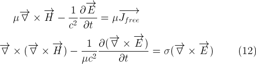
Plane Harmonic Wave Equations in Harmonic Isotropic Linear Stationary (HILS) medium equation 12 \mu\overrightarrow{\triangledown } \times \overrightarrow{H} - \frac{1}{c^2} \frac{\partial \overrightarrow{E}}{\partial t}= \mu\overrightarrow{J_{free}} \\ \\ \overrightarrow{\triangledown } \times(\overrightarrow{\triangledown } \times \overrightarrow{H}) - \frac{1}{\mu c^2} \frac{\partial (\overrightarrow{\triangledown } \times\overrightarrow{E})}{\partial t}= \sigma(\overrightarrow{\triangledown } \times\overrightarrow{E})  \; \; \; \; \;\;\;\; (12)

Then, we replace the right-hand side of equation (11) and the curl of E (from the 3rd Maxwell`s equation) in equation (12)

Plane Harmonic Wave Equations in Harmonic Isotropic Linear Stationary (HILS) medium equation 13 \overrightarrow{\triangledown } \times \overrightarrow{E} = -\frac{\partial \overrightarrow{B}}{\partial t} = -\mu\frac{\partial \overrightarrow{H}}{\partial t} \\ \\ - \overrightarrow{\triangledown}^2 \overrightarrow{H} + \frac{1}{c^2} \frac{\partial^2\overrightarrow{H}}{\partial t^2}= -\sigma\mu\frac{\partial\overrightarrow{H}}{\partial t} \\ \\ \overrightarrow{\triangledown}^2 \overrightarrow{H} -\sigma\mu\frac{\partial\overrightarrow{H}}{\partial t} - \frac{1}{c^2} \frac{\partial^2\overrightarrow{H}}{\partial t^2}= 0  \; \; \; \; \;\;\;\; (13)
Hence, we have obtain the wave equation for H in a HILS medium.

So, we have finally obtained the wave equations for both E and H. That`s what we wanted.


Now, let`s try an additional simplification for the wave equation for E.

let E be in the x-direction,
Plane Harmonic Wave Equations in Harmonic Isotropic Linear Stationary (HILS) medium equation 13-1 \overrightarrow{\triangledown }\cdot \overrightarrow{E} = \frac{\rho_{free}}{\varepsilon_0} \; \; \; ; \;\frac{\overrightarrow{E}}{\left |\overrightarrow{E} \right |}=\widehat{i}  \; \; \; \; ; \; \overrightarrow{\triangledown }\cdot \overrightarrow{E} = \frac{\partial E_x}{\partial x}

Plane Harmonic Wave Equations in Harmonic Isotropic Linear Stationary (HILS) medium equation 13-2 \overrightarrow{\triangledown}(\frac{\rho_{free}}{\varepsilon_0}) = \overrightarrow{\triangledown}(\overrightarrow{\triangledown}\cdot \overrightarrow{E}) = \frac{\partial^2 \overrightarrow{E}}{\partial x^2} \widehat{i} = \overrightarrow{\triangledown}^2 \overrightarrow{E}

We can therefore replace the right-hand side of equation (9) with the result of the above equation

Plane Harmonic Wave Equations in Harmonic Isotropic Linear Stationary (HILS) medium equation 14-15 \center\overrightarrow{\triangledown}^2 \overrightarrow{E} -  \sigma\mu \frac{\partial \overrightarrow{E}}{\partial t} - \varepsilon\mu \frac{\partial^2 \overrightarrow{E}}{\partial t^2} =  \overrightarrow{\triangledown}^2 \overrightarrow{E} \\ \\ \\ \Rightarrow \sigma \frac{\partial \overrightarrow{E}}{\partial t} - \varepsilon \frac{\partial^2 \overrightarrow{E}}{\partial t^2} = 0 \; \; \; \; \; \; \; \; (14)
\\ \\ \\ E_x = E_1 +E_2 e^{-\frac{\sigma}{\varepsilon}t} \; \; \; \; \; \; \; \; (15)

Equation (15) is the solution for Ex that would be obtained from (14).

As E and H are transverse, an example of a solution would be
Plane Harmonic Wave Equations in Harmonic Isotropic Linear Stationary (HILS) medium equation 16 \center\overrightarrow{E} = E_0 e^{i(\omega t-kx)} \widehat{j}\\ \\ \overrightarrow{H} = \frac{k}{\omega\mu}E_0 e^{i(\omega t-kx)} \widehat{k}\\ \\ Z = \left | \frac{E}{H}\right | = \frac{\omega\mu}{k} = \mu c = \frac{1}{\varepsilon c} =(\frac{\mu}{\varepsilon})^{\frac{1}{2}}

where Z is the characteristic impedance.

Monday, December 24, 2012

Magnetic field (B-field) tangential to surface of Superconductor

  • Magnetic field (B-field) is always tangential to the surface of a Superconductor

We are going to prove that magnetic fields (B-fields) are always tangential to the surface of a superconductor.

First, let`s briefly discuss what superconductivity is. Superconductivity is the sudden disappearance of all electrical resistance when the material is cooled below a certain temperature, called the critical temperature. Apart from the disappearance of all electrical resistance, what makes superconductors to be of great interest is that superconductors have extraordinary magnetic properties.

There are 2 types of superconductivity:
  • Superconductivity of type I (discovered by Omnes),
  • Superconductivity of type II (discovered by Bednorz and Muller)

Let`s now look at the properties of superconductors of type I.

Properties of superconductive material of type I

  • There is an absence of the magnetic field (B-field) inside the superconductor. In fact, the B-field is expelled from inside of the material (B = 0 inside - Meissner-Ochsenfeld effect). This is independent of how the transition to the superconductor state occurs. (There is a loss of history) Note that in superconducting alloys, the Meissner-Ochsenfeld effect is not sharp and the field can penetrate the superconductor.
  • There is a persistent current inside the material even in the absence of an electromotive force (battery).
  • There is no magnetization of the material.
  • Current flows along a skin (thickness ~ 10^-7m) around the boundary of the material.

Let`s now explain how the B-field is always tangential to the surface of a superconductor.

From Maxwell`s equations, we know that the divergence of B is zero (div(B) = 0). It follows that the magnetic field lines are continuous and closed. Therefore, the components of B normal to the surface, Bn must be equal on both sides of the surface, that is, both inside and outside the material.

However, from the first property mentioned above, the B-field is zero inside (so, it is also zero outside the material). It follows that the normal component at the external field at the surface outside the superconductor is also zero. This means that the magnetic field lines are tangential to the surface of the superconductor. The magnetic field lines surround the superconductor.


Additionally, as B = 0 inside, this means that the mean density of current = 0. Therefore, there is no magnetization field and no H-field.

Saturday, December 22, 2012

Magnetization in fluid in Quantum Mechanical Case

  • Magnetization in fluid in Quantum Mechanical Case

Previously, we found the equation for magnetization of a fluid in the classical case. Now, let`s find the equation for magnetization of a fluid for the quantum mechanical case.

Here, we consider the fluid to have N spins up (Nup) and N spins down (Ndown). In the presence of an external field B, the energy is given by where the positive z-axis points upwards.

Again, as in the classical case for magnetization of a fluid (Langevin`s equation), the relative probability of having any angle is, from statistical mechanics, exp(-energy/kT).

So,  Magnetization in fluid in Quantum Mechanical Case equation 2and Magnetization in fluid in Quantum Mechanical Case equation 3. If  N is the total number of dipoles, them M is the product of N with the average magnetic moment along the z-axis.


Magnetization in fluid in Quantum Mechanical Case equation 4 - N = N_{up} + N_{down} \\ \\\mu  = \frac{N_{up}(-\mu_{z})  +  N_{down}(\mu_{z})}{N}\\ \\
M = N\mu = N\mu_{z}\frac{e^{\frac{+\mu_{z} B}{kT}} - e^{\frac{-\mu_{z} B}{kT}}}{e^{\frac{+\mu_{z} B}{kT}} + e^{\frac{-\mu_{z} B}{kT}}}\\ \\ M = N\mu_{z}\tanh(\frac{\mu_{z}B}{kT}) \\ \\ M = N\mu_{z}\tanh(u) \; \; ;\; \; u = frac{\mu_{z}B}{kT}

In most normal cases, say, for typical moments, room temperatures, and the fields one can normally get (like 10 000gauss), the ratio represented by u is about 0.02. One must go to very low temperatures to see the saturation. For normal temperatures, tanh(u) can be replaced by u and

Magnetization in fluid in Quantum Mechanical Case equation 5

The graph of M against u for the quantum mechanical case of magnetization in fluids resembles that for the classical case.

Equation for Magnetization in Quantum Fluid graph

When B gets very large, the hyperbolic tangent approaches 1, and M approaches the limiting value (N x the average magnetic moment along the z-axis). So, at high fields, the magnetization saturates. We can see why that is,; at high enough fields, the moments are all lined up in the same direction . In other words, they are all in the spin-down state, and each atom contains the same moment.


Additionally, when we look at the expressions for magnetization in the fluid at room temperature for both the classical and quantum case, we notice that M is proportional to B/T. From this, we can derive Curie`s law which is M = kB/T, where k is a constant.

Wednesday, December 19, 2012

Langevin`s Equations for Magnetization in Classical Fluid

  • Langevin`s Equations for Magnetization in Classical Fluid


Consider a fluid at a temperature T, with dipole moments. As the molecules collide with each other, the magnetic field exerts a mean restoring force. That is, there is a resultant magnetic moment M.

In the absence of a field, the number of randomly oriented molecules satisfy the equation


where N is the total number of dipoles &  is the solid angle (the whole of space).

Consider a sphere, = 4, then the solid angle at is


This can also be shown by the fractional surface area of a surrounding sphere. That is, the area obtained on the surface of the sphere when we are situated at an angle and we moved by an angle d, over the total surface area  of the sphere.


where dN lies between and +d

One assumes that each of the atom has a magnetic moment , which always has the same magnitude but can point in any direction.

The orientation of atomic magnetic dipoles with respect to external magnetic field B give rise to a magnetic potential energy given by , where is the angle between the moment and the field. From statistical mechanics, the relative probability of having any angle is exp(-energy/kT), so angles near zero are more likely than angles near .

Therefore dN is proportional to


where C is the Normalization constant.


Each moment contributes an amount to the magnetization parallel to the field. This is because the components will give zero value because of the symmetry of the problem.  The magnetization resulting from all dipoles within is given by


let so


Performing the integration and re-arranging gives


At normal temperature, cosh(u) can be expanded as


So, at normal temperature,


So, magnetic effects will be noticeable small at lower temperature for the case of classical fluid.

A typical graph of M against u would be as follows:
Langevin`s Equations for Magnetization in Classical Fluid graph
Currently Viewing: Physics Reference |