• Complex Analysis: #8 Zeros of Analytic Functions

Definition 7
Let f : G → ℂ be an analytic function defined in a region G. A point z₀ ∈ G with f(z₀) = 0 is called a zero of the function.

So let z₀ ∈ G be a zero of the analytic function f : G → ℂ. As usual, without loss of generality, we may assume that z₀ = 0. As we have seen, we can choose some r > 0 such that B(0, r) = {z : |z| < r} ⊂ G and

for all such z ∈ B(0, r).

The fact that f(0) = 0 means that c₀ = 0. Let k > 0 be the smallest integer such that c_k ≠ 0. (If c_n = 0 for all n, then f is simply the constant function which is zero everywhere. This is not what we are interested in here so we will assume that some k exists with c_k ≠ 0.) The easiest case is then that k = 1. In this case, we have

and in particular f '(0) = c₁ ≠ 0. Could it be that for every ∈ > 0 there exists a complex number z_∈ with 0 < |z_∈| < ∈ and yet f(z_∈) = 0? But that would imply that

That is impossible, since f '(0) ≠ 0. Therefore we have:


Theorem 14
Let f : G → ℂ be analytic and let z₀ ∈ G be such that f(z₀) = 0 while f '(z₀) ≠ 0. Then there exists an ∈ > 0 such that B(z₀, ∈ ) ⊂ G and the only zero of f in B(z₀, ∈ ) is the single number z₀.

Of course, another way of thinking of these things — and remembering what was done in Analysis II — is to consider f to be a continuously differentiable mapping of G into ℂ, represented as ℝ². The mapping f is then totally differentiable, and the derivative at z₀ is not singular; thus it is a local bijection around z₀.

More generally, we might have k being greater than 1. In any case, the number k is called the order of the zero. A zero of order 1 is also called a simple zero.


Theorem 15
Let f : G → ℂ be analytic in the region G, and let z₀ ∈ G be a zero of f of order k. Then there exists an ∈ > 0 such that in the open disc B(z₀, ∈ ) of radius ∈ around z₀ we have f(z) = (h(z))^k where h : B(z₀, ∈ ) → ℂ is analytic with a simple zero at z₀.

Proof
For sufficiently small ∈ > 0, we can write

say, for z ∈ B(z₀, ∈ ). Here g : B(z₀, ∈ ) → ℂ is analytic, and g(z₀) = c_k ≠ 0. Thus there are k distinct k-th roots of the number g(z₀) = c_k. [For any w ≠ 0 in ℂ we have w = re^iθ say. Then each of the numbers ^k√r · e^{iθ/k + 2πil/k} , for l = 0, . . . , k − 1, is a different k-th root of w.] Let z₁ be one of these k-th roots of g(z₀). Now consider the particular polynomial function ϕ_k'(z) = z^k. We know that ϕ_k is an entire function, and that ϕ_k'(z₁) = kz₁^k−1 ≠ 0, since z₁ ≠ 0. So there is a neighborhood U₁ of z₁, and a neighborhood V₁ of g(z₀), such that ϕ_k : U₁ → V₁ is a bijection [ϕ_k is totally differentiable and non-singular at z₁], with ϕ_k(z₁) = g(z₀). Let ϕ_k⁻¹ : V₁ → U₁ be the inverse mapping. Now choose ∈ > 0 so small that g(B(z₀, ∈ )) ⊂ V₁. Then take h(z) = (z − z₀) · ϕ_k⁻¹(g(z)). This defines a function h : B(z₀, ∈ ) → ℂ which satisfies our conditions.[As in real analysis (the proof is the same here in complex analysis) we have the rule that if ϕ is an invertible differentiable function (with non-vanishing derivative), then ϕ⁻¹ is also differentiable, with derivative (ϕ⁻¹) '(z) = 1/ϕ '(ϕ⁻¹(z)).]


Theorem 16
Again let f : G → ℂ be analytic in the region G, and let z₀ ∈ G be a zero of order k. Then there exists an ∈₀ > 0 and an open neighborhood U_∈0 ⊂ G of z₀ with f(U_∈0) = B(0, ∈₀). Within U_∈0 ,z₀ is the only zero of f, and if w ≠ 0 in B(0, ∈₀) then there are precisely k different points v₁, . . ., v_k in U_∈0 with f(v_j) = w, for all j.

Proof
Since f is continuous and B(0, ∈₀) is open, it follows that U_∈0 = f ⁻¹(B(0, ∈₀)) is also open, regardless of how the number ∈₀ > 0 is chosen. So we begin by choosing an ∈₁ > 0 sufficiently small that we can use theorem 15 and write f(z) = (h(z))^k, for all z ∈ B(0, ∈₁). Since h has a simple zero at z ₀, and therefore the derivative at z ₀ is not zero (h '(z ₀) ≠ 0), there exists a neighborhood of z ₀ such that h is a bijection when restricted to the neighborhood. So let ∈ > 0 be chosen sufficiently small that B(0, ∈) is contained within the corresponding neighborhood of 0. Finally, with this ∈ , we take ∈₀ = ∈^k . Then if w ≠ 0 in B(0, ∈₀), we have k different k-th roots of w, lets call them u₁, . . ., u_k. They are all in B(0, ∈). Therefore each has a unique inverse under h, namely v_j = h⁻¹(u_j), for j = 1, . . . , k. Is it possible that some other point, v say, not equal to any of the v_j, also is such that f(v) = (h(v))^k = w? But then h(v) would also be a k-th root of w, not equal to any of the u_j, since after all, h⁻¹ is a bijection when restricted to B(z₀, ∈₀). This is impossible, owing to the fact that there are only k different k-th roots of w.

Complex Analysis: #7 Standard Theorems of Complex Analysis

• Complex Analysis: #7 Some Standard Theorems of Complex Analysis

Combining the last two theorems, we have:

Corollary (Goursat’s Theorem)
The derivative of every analytic function is again analytic. Thus every analytic function has arbitrarily many continuous derivatives.

We can also complete the statement of theorem 3


Theorem 10 (Morera’s Theorem)
Let G ⊂ ℂ be a region and let f : G → ℂ be continuous such that ∫_γ f(z)dz = 0, for all closed paths which are the boundaries of triangles completely contained within G. Then f is analytic.

Proof
According to theorem 3, there exists an antiderivative F : G → ℂ, with F' = f. Thus, by Goursat’s Theorem, f is also analytic.



Theorem 11 (Cauchy’s estimate for the Taylor coefficients)
Again, let f : G → ℂ be analytic, z₀ ∈ G, r > 0 is such that D(z₀, r) = {z : |z − z₀| ≤ r} ⊂ G, and

for all z ∈ D(z₀, r). Since f is continuous and D(z₀, r) is compact, we must have |f| being bounded in D(z₀, r). Let M > 0 be such that |f(z)| ≤ M for all z ∈ D(z₀, r). Then we have

Definition 5
Let the function f : ℂ → ℂ be defined throughout the whole complex plane, and let it be analytic everywhere. Then we say that f is an entire function.


Theorem 12
A bounded entire function is constant.

Proof
Assume that the entire function f : ℂ → ℂ is bounded with |f(z)| ≤ M say, for all z ∈ ℂ, where M > 0 is fixed. Thus |c_n| ≤ M/rⁿ = 0 for all r > 0. This can only be true if c_n = 0 for all n > 0.

Definition 6
A field is called algebraically closed if every polynomial within the field of degree greater than or equal to one has a root.


Theorem 13 (The Fundamental Theorem of Algebra)
ℂ is algebraically closed.

Proof
Let f(z) = ∑a_kz^k, (with k = 0, . . .,n), with n ≥ 1 and a_n ≠ 0 be a polynomial of degree n. Looking for a contradiction, we assume that there is no root, that is, f(z) ≠ 0 for all z ∈ ℂ.

For z ≠ 0, we have

Note that for a and b arbitrary numbers, we have |a| = |a + b − b| ≤ |a + b| + |b| or |a + b| ≥ |a| − |b|, and more generally, |a + b₁ + · · · + b_n| ≥ |a| − |b₁| − · · · − |b_n|.

Since |a_n|/2 remains constant, |zⁿ| · |a_n|/2 becomes arbitrarily large, as |z| → ∞. Therefore |f(z)| → ∞ when |z| → ∞. That is to say, if M > 0 is given, then there exists an r > 0 such that |f(z)| > M for all z with |z| > r. That is, |1/f(z)| < 1/M for |z| > r. Now, since f(z) ≠ 0 always, and f (being a polynomial) is an entire function, we have that 1/f is also an entire function. It is bounded outside the closed disc D(0, r), but since the function is continuous, and D(0, r) is compact, it is also bounded on D(0, r). Thus it is bounded throughout ℂ, and is therefore constant, by theorem 12. Therefore, the polynomial f itself is a constant function. This contradicts the assumption that f is of degree greater than zero.

• Complex Analysis: #6 Power Series

Definition 4
A power series is a sum of the form

where (a_n)_n∈ℕ0 is some arbitrary sequence of complex numbers and z₀ is a given complex number. (ℕ₀ is the set of non-negative integers)

So the question is, for which z does the power series converge? Well it obviously converges for z = z₀. But more generally, we can say the following.


Theorem 8
Let the power series ∑a_n(z − z₀)ⁿ, (with n = 0, . . .,∞) be given. Then there exists 0 ≤ R ≤ ∞, the radius of convergence, such that

1. The series is absolutely convergent for |z − z₀| < R, and uniformly convergent for |z − z₀| ≤ ρ, for 0 ≤ ρ < R fixed. 
2. It diverges for |z − z₀| > R.
3. The radius of convergence is given by 1/R = lim_n→∞ sup ⁿ√|a_n|. 
4. The function given by f(z) = ∑a_n(z − z₀)ⁿ, (with n = 0, . . .,∞) is analytic in the region |z − z₀| < R. For each such z, the derivative is given by the series f '(z) = ∑na_n(z − z₀)^n-1, (with n = 1, . . .,∞), and the radius of convergence of this derivative series is also R. 

Proof
Parts 1 and 2 are proved in the analysis lecture. For 3, let |z − z₀| < ρ < R with 1/R = lim_n→∞ sup ⁿ√|a_n|. Thus there exists some N₀ ∈ ℕ with √|a_n| < 1/R for all n ≥ N₀. That is, |a_n| < 1/Rⁿ. Therefore

with ρ/R < 1. This is a geometric series which, as is well known, converges. On the other hand, if |z − z₀| ≥ ρ > R then there exist arbitrarily large n with ⁿ√|a_n|  > 1/R. That is,  |a_n| > 1/Rⁿ or

So the series cannot possibly converge, since the terms of the series do not converge to zero.

As far as part 4 is concerned, it is clear that lim_n→∞ sup ⁿ√|na_n| = lim_n→∞ sup ⁿ√|a_n| since lim_n→∞ sup ⁿ√n = 1. So let f₁(z) = ∑na_n(z − z₀)^n-1, (with n = 1, . . .,∞), be the function which is defined in the region |z − z₀| < R. We must show that f is analytic here, with f ' = f₁. To simplify the notation, let us assume from now on that z₀ = 0. Choose some complex number w with |w| < R. We must show that the derivative of f exists at w, and it equals f₁(w).

To begin with, we write

So take some ρ with |w| < ρ < R and we restrict ourselves to examining complex numbers z with |z| < ρ. Furthermore, choose ∈ > 0. We must show that there exists a δ > 0 such that if 0 < |z −w| < δ then

(Remember that the series is absolutely and uniformly convergent in the closed disc with radius ρ.) Thus for some N₁ ∈ ℕ, the “tail” of the series beyond N₁ sums to something less than ∈ /3. Similarly, the series defining f₁ is absolutely and uniformly convergent in this disc. Therefore take N₂ to be sufficiently large that

for all n ≥ N₂. Let N be the larger of N₁ and N₂. Finally we must determine the number δ. For this, we note that since S_n is just a polynomial, and thus analytic, we have a δ > 0 such that

for all z with |z − w| < δ. In particular, if necessary, we can choose a smaller δ to ensure that such z are in our disc of radius ρ. The fact that

Theorem 9
Let f : G → ℂ be an analytic function defined in a region G, and let z₀ ∈ G be given. Then there exists a unique power series ∑a_n(z − z₀)ⁿ, (with n = 0, . . .,∞) whose radius of convergence is greater than zero, and which converges to f(z) in a neighborhood of z₀.

Proof
Let r > 0 be sufficiently small that B(z₀, r) = {z ∈ ℂ : |z − z₀| < r} ⊂ G. In fact, we will also assume the r is sufficiently small that z ∈ G for all z with |z − z₀| = r. Once again, in order to simplify the notation, we will assume that z₀ = 0. That is to say, we will imagine that we are dealing with the function f(z − z₀) rather than the function f(z). But obviously if the theorem is true for this simplified function, then it is also true for the original function. According to theorem 7, for |z| < r we then have

Here are a few points to think about in this proof.

• The third equation is true since |z/ζ| < 1, and thus the sum is absolutely convergent. 
• The fifth equation is true since the partial sums are uniformly convergent, thus the sum and integral operations can be exchanged. 
• Although the function f(ζ)/ζⁿ⁺¹ is not differentiable at zero, it is defined and continuous on the (compact) circle |ζ| = r. Thus, although c_n is not always zero, still it is always a well defined complex number, for all n. 
• It looks like c_n might vary with r. But this is not the case. Theorem 8 implies that f⁽ⁿ⁾(0) = n!c_n, for all n, and this is certainly independent of r. 
• The power series converges to f(z) at all points of B(z₀, r).

• Complex Analysis: #5 Cauchy`s Integral Formula

Theorem 6
Let G ⊂ ℂ be a region and let f : G → ℂ be analytic. Take z₀ ∈ G and r > 0 so small that {z ∈ ℂ : |z − z₀| ≤ r} ⊂ G. Furthermore, let |a − z₀| < r. Then

converges to the constant number f '(a) in the limit as ∈ → 0. On the other hand, the path length around the circle, and the tangent vector to this path, approach zero as ∈ → 0. Thus in the limit, the first integral is zero. As far as the second integral is concerned, we have

A relatively trivial implication is the following theorem.


Theorem 7
The same assumptions as in Theorem 6. But this time take z₀ to be the central point of the circle. Then

So this is just a kind of “mean value theorem” for analytic functions. It shows quite clearly the difference between real analysis and complex analysis. In real analysis, we can make a smooth change in a function, leaving everything far away unchanged, and the function remains nicely differentiable. But in complex analysis, the precise value of the function is determined by the values on a circle, perhaps far away from the point we are looking at. So a change at one place implies that the whole function must change everywhere in order to remain analytic.

• Complex Analysis: #4 Cauchy`s Theorem (simplest version)

Theorem 1
Let G ⊂ ℂ be a region, and assume that the function f : G → ℂ has an antiderivative (auf deutsch: Stammfunktion) F : G → ℂ with F' = f. Let γ be a closed path in G (that is, a continuous, closed, piecewise continuously differentiable path). (Closed means that γ(t₀) = γ(t₁).) Then ∫_γ f(z)dz = 0.

Proof

Since every polynomial has an antiderivative, it follows that the path integral around a closed path for any polynomial is zero.

Of course this is all a bit too trivial. So let’s call the following theorem the simplest version of Cauchy’s integral theorem.


Theorem 2
Let Q be a (solid) triangle in the complex plane. Assume that Q ⊂ G ⊂ ℂ, and take f : G → ℂ to be an analytic function. Let γ be the closed path traveling around the three sides of Q. Then ∫_γ f(z)dz = 0.

Proof
We may assume that γ begins and ends in a corner of Q — for example the “lowest” corner γ in the complex plane. If the lower side of Q is parallel to the real number axis, then take the right-hand corner on that side. Let us now divide the sides of Q in half, connecting the half-way points with straight line segments, thus creating four equal sub-triangles, Q₁, . . . , Q₄. Let γ_j be the path traveling around the boundary of Q_j, for j = 1, . . . , 4. Again we may assume that each γ_j begins and ends in the bottom right corner of it’s triangle. So we have

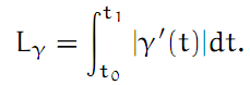
Assume further that each of these paths is parameterized in the simplest way possible, so that |γ'| = 1 and |γ_j'| = 1 for all the j. Therefore L_γ is the sum of the lengths of the three sides of the triangle Q, and L_γj = L_γ/2 for each of the j.

Let’s say that γ₁ is one of the numbers between one and four such that the value of

is the greatest. Then we certainly have

The next step is to concentrate on the triangle Q_j1. As with Q, we subdivide Q_j1 into four equal sub-triangles and we take paths around their boundaries. Choose Q_j2 to be one of these sub-triangles of Q_j1 which is such that the value of

is the greatest. Here γ_j2 is the path around the boundary of Q_j2. Now we have L_γj2= L_γ/4, and

This whole process is continued indefinitely, so that we obtain a sequence of triangles, becoming smaller and smaller, converging to a point, z₀ ∈ Q say,

Q ⊃ Q_j1⊃ Q_j2 ⊃ · · · → z₀ ∈ Q. 

For each n we have L_γjn= L_γ/2ⁿ and

But we have assumed that f is analytic, in particular it is differentiable at the point z₀. Thus we can write

f(z) = f(z₀) + f '(z₀)(z − z₀) + χ(z),

for points z in G, where χ : G → ℂ is a continuous function with

So let ∈ > 0 be arbitrarily given. Then there exists some δ > 0 such that |χ(z)| < |z − z₀| for all z with 0 < |z − z₀| < δ.

Now we need only choose n so large that |z − z₀| < δ for all z ∈ Q_jn. For such z we have

On the other hand, again since the length of L_γjnis L_γ/2ⁿ, we have

Bearing in mind Theorem 1 (and remembering that f '(z₀) is simply a constant complex number), we conclude that

Since ∈ was arbitrary and L_γ remains constant, we conclude that ∫_γ f(z)dz = 0.

But now Theorem 2 can be turned around, and we obtain (almost) the converse.


Theorem 3
Assume G ⊂ ℂ is a region and f : G → ℂ is a continuous function. Assume furthermore that for any solid triangle Q contained in G we have ∫_γ f(z)dz = 0, where γ is the path around the triangle. Then f has an antiderivative in every open disc contained in G. That is, let U = {z ∈ ℂ : |z − z_*| < r} be some such disc, where z_* is a complex number (the middle point of the disc) and r > 0 is the radius of the disc. Then there exists F : U → ℂ with F'(z) = f(z) for all z ∈ U.

Proof
By replacing f with the function f_*, where f_*(z) = f(z − z_*), we obtain the situation that z_* = 0. Clearly, if the theorem is true for f_*, then it is also true for f. Therefore, without loss of generality, we may simply assume that z_* = 0.

Within U the function F is defined to be

Here, α_z is the straight line from 0 to z, that is, α_z(t) = tz. To show that F really is an antiderivative to f in U, let z₀ be some arbitrary point of U and let z be some other point of U. Let β be the straight line connecting z₀ to z. That is, β(t) = (1 − t)z₀ + tz. Being a triangle, the integral of f around the path from 0 out to z, then from z to z₀ then from z₀ back to 0 must itself be zero. That is,

Looking at the definition of the path integral, we see that

Combining this theorem with Theorems 1 and 2, we see that if D ⊂ G is a closed disc, and γ is the circle of it’s boundary, then  ∫_γ f(z)dz = 0, for any analytic function defined in the region G. In fact, if γ is any (piecewise continuously differentiable and continuous) closed path contained within this disc-like G, then  ∫_γ f(z)dz = 0. For example we can look at a rectangle [a, b] × [c, d] contained within G. Since the rectangle can be taken to be a union of two triangles, attached along one side, we see that also the path integral around the rectangle must be zero.

More generally, the following theorem will prove to be useful.


Theorem 4
Let Q = {x + iy : 0 ≤ x, y ≤ 1} be the standard unit square in ℂ. Take ζ to be the standard closed path, traveling around the boundary of Q once in a counterclockwise direction, beginning and ending at 0. Assume that a continuously differentiable mapping ϕ : Q → ℂ is given, such that ϕ(Q) ⊂ G, a region where an analytic function f : G → ℂ is defined. Let γ = ϕ ◦ ζ be the image of ζ under ϕ. Then ∫_γ f(z)dz = 0.

Proof.
Since Q is compact, ϕ(Q) is also compact. Therefore it can be covered by a finite number of γ open discs in G. But Q can now be partitioned into a finite number of sub-squares Q₁, . . ., Q_n such that ϕ(Q_j) is in each case contained in a single one of these open discs. The theorem then follows by observing that the path integral around each of these sub-square images must be zero.

 Note:-
[The inverse images of the open discs in Q form a finite open covering V₁, . . ., V_m of Q. A sequence of partitions of Q can be obtained by cutting it along horizontal and vertical lines spaced 1/n apart, for each n ∈ ℕ. Can it be that for each of these partitions, there exists a sub-square which is not contained completely in one of the open sets V_k? But that would mean that there exists a limit point q ∈ Q such that for every ∈ > 0, there are infinitely many of these sub-squares contained within a distance of from q. However q ∈ V_k, for some k, and since V_k is open, there exists an ∈-neighborhood of q contained entirely within V_k, providing us with the necessary contradiction.]

A special case is the following.


Theorem 5
Let D₁ and D₂ be closed discs in ℂ such that D₂ is contained in the interior of D₁. Let γ_j be the closed path going once, counterclockwise, around the boundary of D_j, j = 1, 2. Let G ⊂ ℂ be a region containing D₁\D₂ and also containing the boundary of D₂. Assume that f : G → ℂ is analytic. Then ∫_γ1 f(z)dz = ∫_γ2 f(z)dz.

Proof
The annulus between D₂ and D₁ can be taken to be the image of the unit square under a continuously differentiable mapping.

A convenient notation for this situation is the following. Let γ : [0, 1] → ℂ be the path γ(t) = z₀ + re^2πit . Then we simply write

With this notation, we can say that if the analytic function f is defined in a region containing the annulus {z ∈ ℂ : r ≤ |z| ≤ R}, then we must have

• Complex Analysis: #3 Path Integrals

Let t₀ < t₁ be two real numbers. Then a continuous mapping γ : [t₀, t₁] → G ⊂ ℂ is a path in the region G of ℂ. In the analysis lecture we learned that γ is rectifiable if a number L exists such that for all ∈ > 0, a δ > 0 exists such that for every partition t₀ = a₀ < a₁ < · · · < a_n = t₁ which is such that a_j+1 − a_j < δ for all j, we have

Let γ(t) = γ_r(t) + iγ_i(t), where γ_r, γ_i: [t₀, t₁] → ℜ are real-valued functions. Then we say that the path is continuously differentiable if both the functions γ_r and γ_i are continuously differentiable. In this case, γ' = γ_r' + iγ_i' is also a path in ℂ. [Thinking in terms of 2-dimensional real geometry, we can say that γ'(t) is the "tangent vector" to γ(t).] We also learned that continuously differential paths are always rectifiable, and we have

All of this has already been dealt with in the analysis lecture. For us now, the interesting thing is to think about path integrals through a region where a complex-valued function is given.


Definition 3
Let G ⊂ ℂ be a region, and let f : G → ℂ be a function. Furthermore, let γ : [t₀, t₁] → G be a differentiable path. Then the path integral of f along γ is

assuming it exists.

The integral here is simply the sum of the integrals over the real and the imaginary parts. It is not necessary to assume that γ is continuously differentiable, but we will assume that it is piecewise continuously differentiable. That is, there is a partition of the interval [t₀, t₁] such that it is continuously differentiable along the pieces of the partition. So from now on, we will (almost) always assume that all paths considered are piecewise continuously differentiable.

As an exercise (using the substitution rule for integrals), one sees that the path integral does not depend on the way the path is parameterized. The simplest case is that, say γ(t) = t. Then (taking t from 0 to 1) we just have ∫_γ f(z)dz = ∫₀¹ f(t)dt. Almost equally simple is the case that γ(t) = it. Then we have ∫_γ f(z)dz = i∫₀¹ f(it)dt.

Increasing the complexity of our thoughts ever so slightly, we arrive at the first version of Cauchy’s integral theorem.

• Complex Analysis: #2 Analytic Functions

Definition 1
Any non-empty connected  open set G ⊂ ℂ will be called a region.

(Recall that in ℜ², every open connected subset is also path-connected.) So we will generally be interested in functions f : G → ℂ defined in regions.

Definition 2
Let f : G → ℂ be given, and let z₀ ∈ G. If

exists, then it is the derivative of f at z₀. The function f will be called analytic in G if it is defined, and has a continuous derivative everywhere in G. The word holomorphic is also used, and it is synonymous with the word analytic.

As in real analysis, we have the simple rules for combining the derivatives of two functions f and g:

Nevertheless, there is a very big difference between the idea of a derivative in complex analysis, and the familiar derivative in real analysis. The reason for this is that a common limit must exist, regardless of the direction with which we approach the point z₀ in the complex plane. This leads to the Cauchy-Riemann differential equations.

Looking at the definition of the complex derivative, one immediately sees that it is really a special version of the total derivative (as in analysis 2) in ℜ². Thus, for ξ ∈ ℂ sufficiently small (that is |ξ| small), we have

f(z₀ + ξ) = f(z₀) + Aξ + |ξ|ψ(ξ), 

where A is a 2 ×2 real matrix, and lim_ξ→0 ψ(ξ) = 0. But what is A? It represents multiplication with the complex number f '(z₀) = a + ib, say. That is,

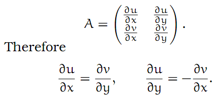
So what are these real numbers a and b? Let f(z) = u(z) + iv(z), where u, v : G → ℜ are real functions. Then writing z = x + iy, we have f(x + iy) = u(x + iy) + iv(x + iy). Identifying ℂ with ℜ², we can consider the partial derivatives of u and v. Since A is simply the Jacobi matrix of the mapping f at the point z₀, we must have

These are the Cauchy-Riemann equations. Another way to express this is to simply say that we must have

Thinking in geometrical terms, we see that if f is analytic, then it is a conformal mapping, at least at the points where f ' is not zero. That means that, locally, the mapping preserves angles. Looked at up close, the mapping is

Of course, as we have already seen, the rotation preserves orientation. Thus it is an element of the group SL₂ (R).

Another interesting detail is that the real and imaginary parts of an analytic function are themselves harmonic functions. Anticipating a later conclusion, let us assume that the parts of the analytic function f = u + iv are twice continuously differentiable. Since ∂u/∂x = ∂v/∂y and ∂u/∂y = −∂v/∂x, we have

Or, expressed in another standard form of notation,

u_xx + u_yy  = ∆u = 0. 

Here, ∆ is the Laplace operator. Similarly, we see that ∆v = 0.

All of this shows that we cannot simply choose any old smooth function f : G → ℂ and expect it to be analytic. On the contrary, there is a very great “rigidity”, which means that most smooth functions — even though they may be partially differentiable when considered as mappings of 2-dimensional Euclidean space — are not complex differentiable.


Examples

1. The first example is the nice and smooth function f(z) = f(x + iy) = x² + y². Here u_x = 2x and v_y = 0. But according to the Cauchy-Riemann equations, we must have u_x = v_y; that is, x = 0. This only holds along a single line in the complex plane ℂ. Therefore it certainly can’t hold in any region of ℂ (since regions are defined to be open), and thus f, despite all appearances of being a nice function, is definitely not analytic.



2. Having been cautioned by the previous example, let us try to construct an analytic function. For example, let us assume that u(x + iy) = x. What possibilities are there for v(x + iy)? Since u_x = 1 = v_y and v_y = 0 = v_x, it is clear that the only possibility is v(x + iy) = y + constant. So this is just the rather boring function f(z) = z + constant.



3. Thinking more positively, we have just seen that the simplest non-trivial polynomial, namely f(z) = z, is analytic throughout ℂ. Of course the simplest polynomial, f(z) = constant, is also analytic. But then, noting that we can use the sum and product rules for differentiation in complex analysis, we see that any arbitrary complex polynomial is analytic throughout ℂ. Indeed, z⁻ⁿ is also analytic (in ℂ \ {0}) for any n ∈ ℕ.